Recursive Functions in Python — A Visual Walk-Through

“Pete and Repete Were Sitting on a Wall…”

If you don’t know the rest of the joke, it goes like this:

“…Pete fell off. Who was left?”
(Answer ‘Repete’)
“OK, if you insist. Pete and Repete were sitting on a wall…”

See, it’s funny because you just keep going, saying the same thing over and over again, simply repeating yourself, on an on, ad nauseam, until the victim simply stops participating, which means you win.

But this isn’t a blog post about dad jokes. This one talks about recursion.

Play it on repeat. You’ll thank me later.

Rapid Recursion Review

Technically, recursion is one of the primary reasons we write programs in the first place. It’s the ability to write out a set of steps and do them over and over again until a certain condition has been met. For example, I want to count from 0 to 9 — you know, the hard stuff.

Fantastic use of print statements! Take note.

If this code is executed, it will produce the following output:

Exciting stuff…

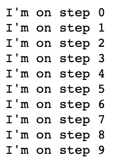
What we’ve done is write a recursive loop that takes an input and modifies it until the stop condition (x = 10) has been reached. The first thing the loop does is evaluate if the stop condition has been met. If not, it runs the code beneath. If so, it moves to the next block of code, if applicable. If you’ve done even basic introductory programming, you’ve probably already dealt with a fair amount of recursion.

Other than typical debugging stuff, the main thing you have to watch out for with recursion is setting the right stop condition or conditions such that the code will, at some point, stop. Say, for example, I made one, teeny tiny little error in the code above and accidentally left out the + sign in the last line.

It’s only one character difference. What’s the worst that could happen?

When this code is run, this is the result:

Pete fell off. Who’s left?

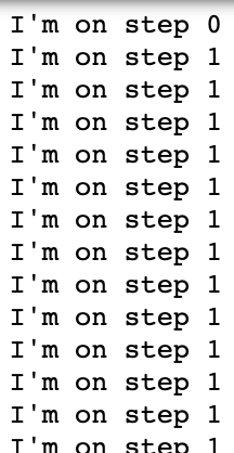
This code will continue to run into infinity, or until the computer dies, the power goes out, or you interrupt the kernel (take your pick). So infinite recursion / infinite loops are typically things to avoid in programming. You have to make sure you have a stop condition defined, and that your stop condition will be met at some point.

Recursive Functions

Recursive functions take this concept up a notch. Rather than a loop that runs inside a function, they are functions that evaluate data and, unless a stop condition is met, they do some modification to the data and then call **themselves** on the modified data.

Let’s turn my counting program into a recursive function to see how this would work:

I added some spacing print statements to help readability of the output

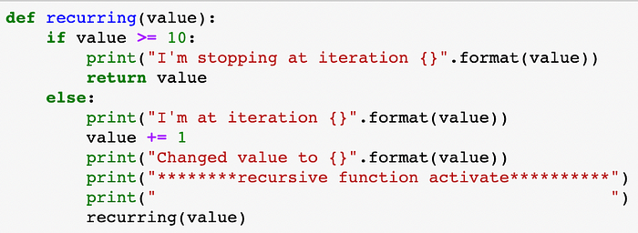
This is now a function I can call, pass in a value, and it will run until the stopping condition is met. Say I execute the following:

Or I could have just used recurring(0) — but why?

This code, with the function as defined above, produces the following output:

Behold, the glory of well-formed print statements!

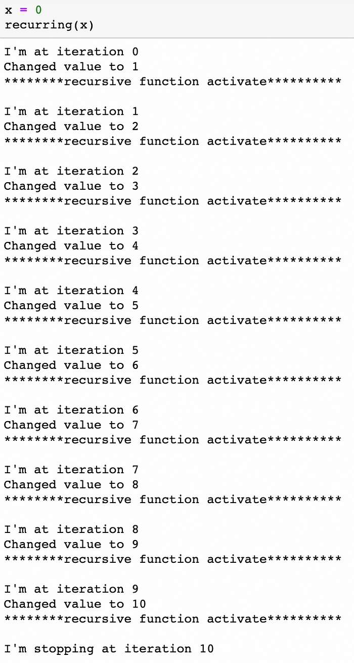
So you can do counting in a loop, or you can do counting with a recursive function. Neither of these are particularly real-world examples, but do you understand how they both worked? Could you diagram the logic?

And just what *can* we do with this in a real-world application? How does recursion work in Python if you are trying to do more than one operation on your data?

Recursive Functions in the Real World

Recursive functions have all kinds of uses, one of which is in writing decision tree algorithms. In a basic scenario, you take input data at what we’ll call the top level “node”, evaluate it, split it by some metric into two additional child nodes that then perform the same exact evaluation. Doing this in a loop inside a function would mean keeping track of a lot of nearly identical variables at each iteration and writing a lot of if / else statements. But using a recursive function really simplifies the coding part, if you understand how the recursion is going to work.

Here’s a basic pseudocode for a decision tree. Note that, just like a loop and our simple recursion function example, the evaluation of whether a stop point has been met or not is the *first* thing the function does:

Evaluate if stopping criteria has been met
If so
* Return the final output
If not
* Split the data into L and R
* Run this function on the L data
* Run this function on the R data
* Do something with the results
* Return the results

While this is helpful, I found that producing a visualization of the process actually really helped me understand what would happen when Python executed the code. Let’s start at the top node — we’ve given it two sets of data (xTr for training data observations, yTr for training data labels).

Let’s assume the first time we run this code, the stopping condition is not met. Therefore, the second part of the function is executed. First the data is split into L and R (for left and right nodes) subsets. Then we call our recursive function on the L data.

To the left.

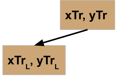
Here’s where the first point of “a-ha” came for me. Python is an interpreted language, meaning it’s going to run one line of code at a time, and does not move to the next one until the one it’s running is finished. So once the first node kicks off the function on its L data, it’s going to be paused and wait for that result to be returned before it moves onto the next step and runs the code on the R data.

So now we move onto the second node. It checks to see if the stop criteria has been met, and we will again assume it has not. Therefore, it is going to do the same thing that the first node did: split the data, then call this function on the L data, creating another node.

To the left, to the left.

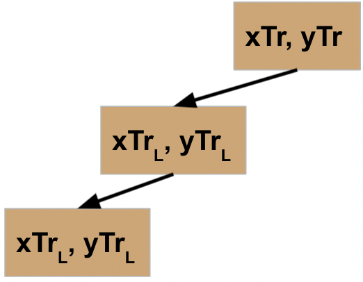
So now, the first and second node are both in a state of waiting for their code to finish executing.

Let’s assume the same thing happens when you get to the third split (fourth node), and it’s not until the fourth split that you finally reach the stopping condition. For a decision tree, once this criteria is met, it typically will return a prediction value.

To the left, to the left, to the left, to the left.

Since this final node does **not** include calling the function again, it is now finished (which is referred to as a “leaf” node). It returns the value to the function that called it.

Now kick (it back).

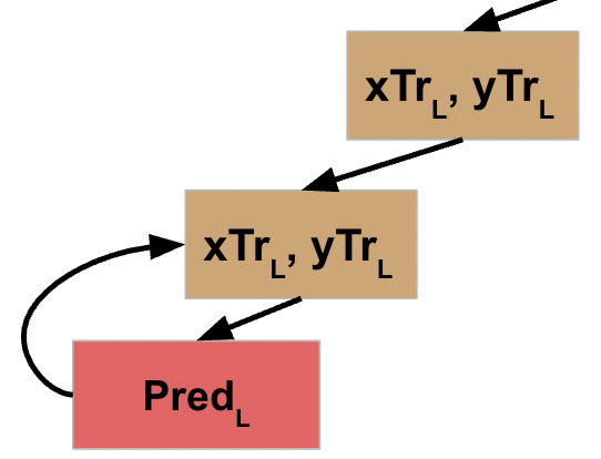
This action completes the line of code that initiated action on the L data, so the prior node is now able to move to the next line of code, which calls the function on the R data for this node. We will assume this node also meets the stopping criteria, so returns the prediction for the R data.

To the right.

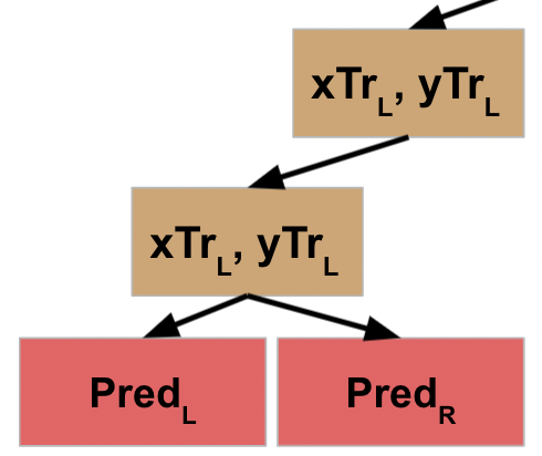
This value gets returned to the prior node, which is now able to execute the next line of code.

Now kick (it back)

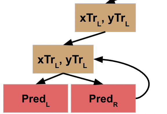
If you’ll go back to the pseudocode, you’ll note that this does something with the output of the L and R functions, and then returns *that* result to the node that called it.

Now kick, now kick…

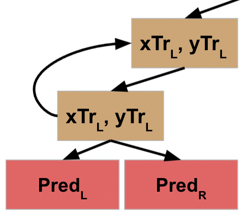
This completes the processing of the L data for *that* node, which means it can move on to its R data.

To the right, to the right.

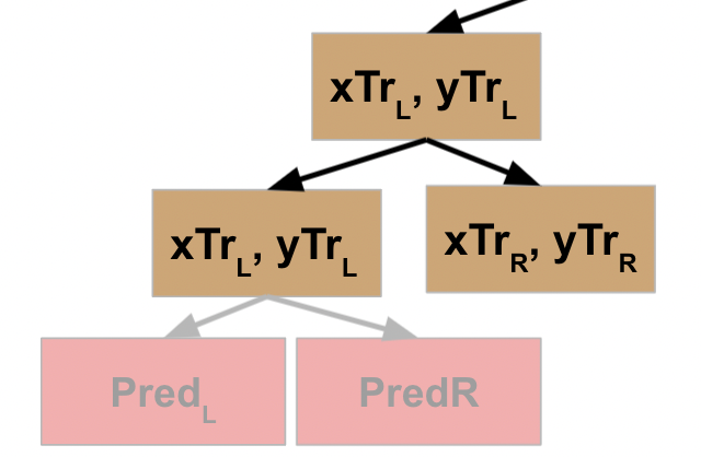
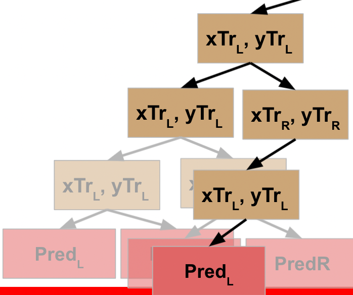
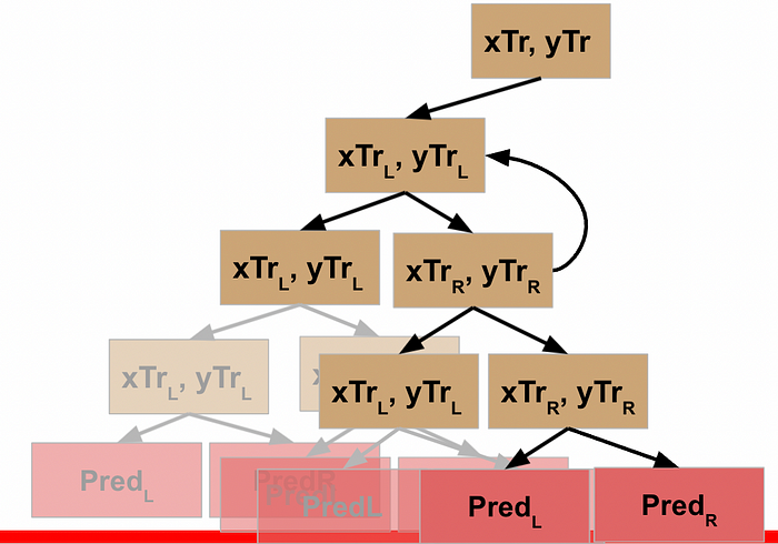
This node evaluates the R data, which does not meet the stopping criteria, so it follows the pseudocode logic again, meaning it splits this data into L and R and executes the function against the L data. This data *does* meet the stopping criteria, and so this generates a prediction / leaf node for the L data…

To the left.

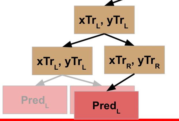
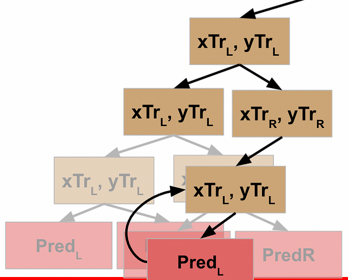
…which returns to result to the prior node, which can then run the function on its R data…

Now kick, now kick, now kick.

To the right, to the right, to the right.

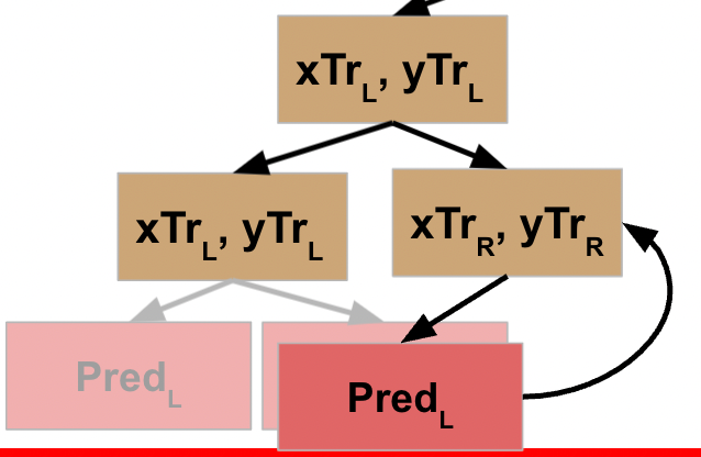
…which returns the result back to the previous node…

Now kick, now kick, now kick, now kick…

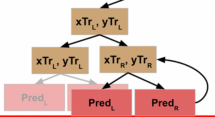
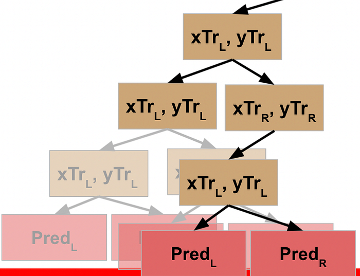
…and allows *this* node to take the results of the L and R processing and return that to its parent node.

Now kick, now kick, now kick, now kick, now kick… uh oh, we may be stuck.

Now **this** node has the results from its L and R function calls, so **it** can write these results back to its parent node.

OK, now you should be able to walk it by yourself from this point.

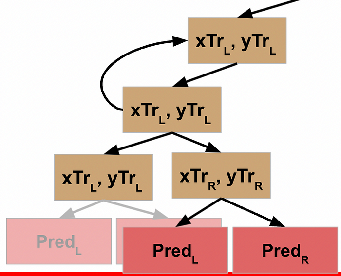
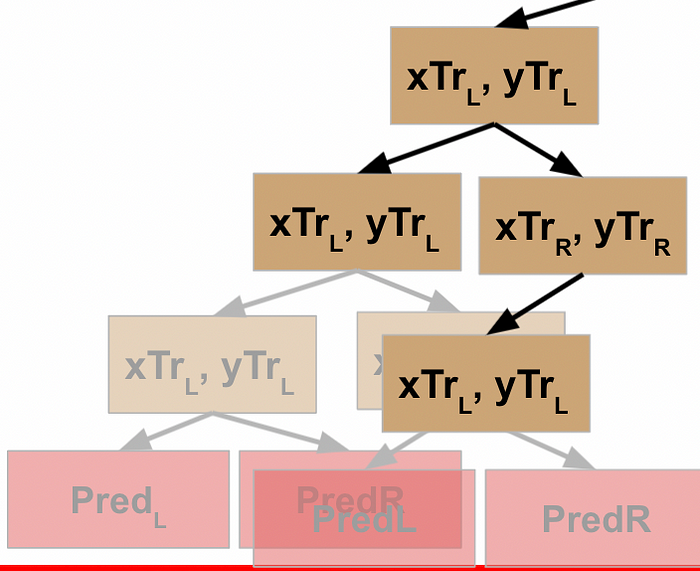
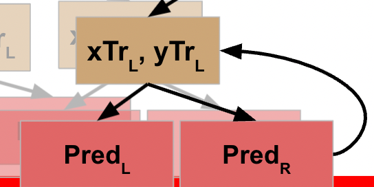
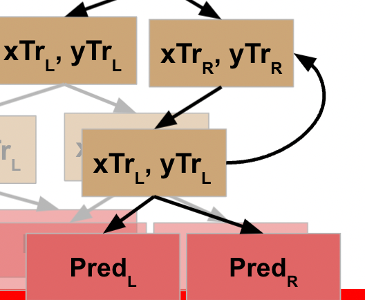
This node has now received the results from its function call on its L data, so it goes to the next line of code and runs the function on the R data.

Rather than explicitly call out the rest of this, I’ll just show the visuals for each step until we get all the way back to the root node of our decision tree.

To the left, to the right, now kick, now kick, now walk it by yourself, now walk it by yourself.

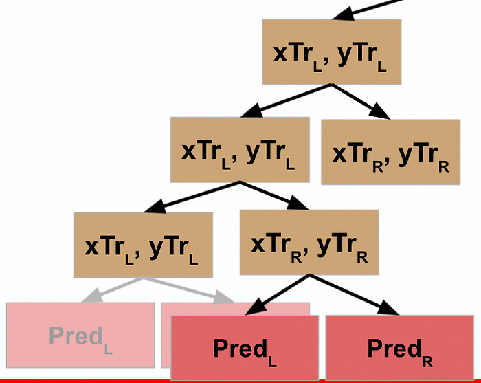
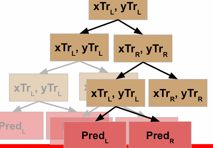
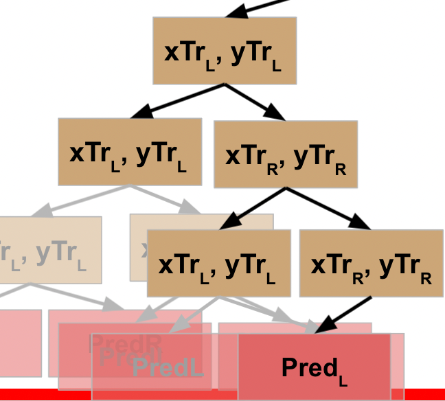
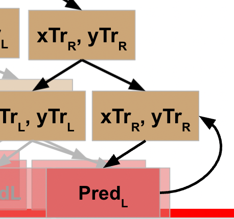
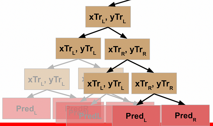
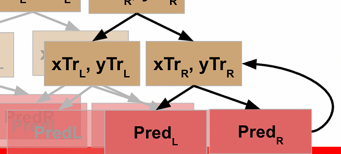
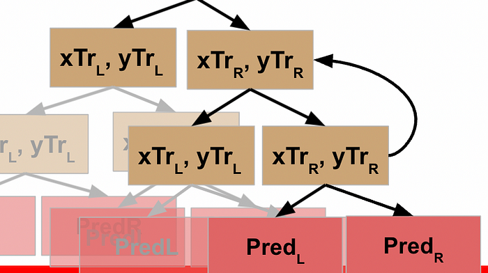
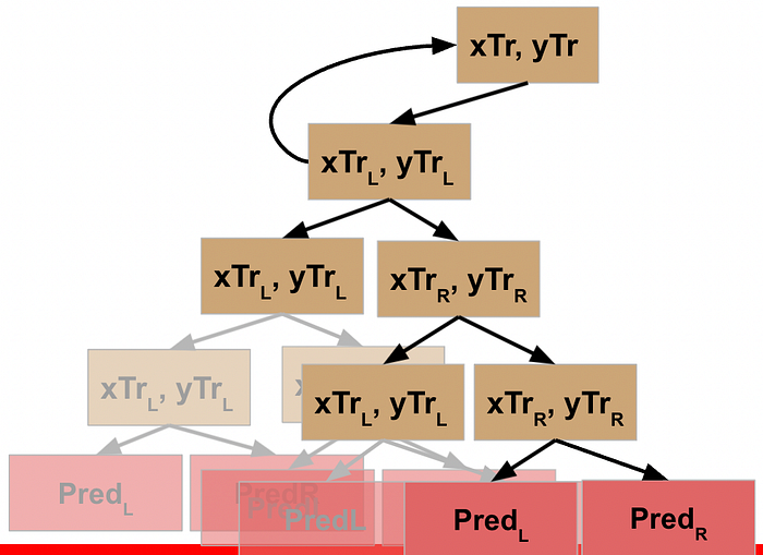
WHEW! Now we’ve made it back to our root node, what happens?

Well, what got returned to the root node was the result of it running the function on its L data. So just like every other node, the root node now moves to the next line of code and repeats the function on the R data.

I’ll spare you the step by step, but one last visual might help put this into perspective:

Down, down, do your dance, do your dance…

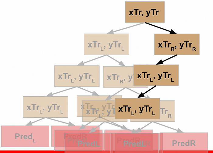
This continues until every node has completed data processing for its L and R data and produced a leaf node at the bottom of the tree.

Summary and Key Points

Recursion in programming is a powerful tool, and using a recursive function can simplify coding even further assuming you have a repetitive set of steps to be executed on similar data across multiple splits. An important thing to ensure is that you have one or more appropriate stop criteria defined at the beginning of the function so that you don’t end up with an infinitely looping set of functions. Recursive functions in Python, because it is an interpreted language and will run one line of code at a time by default, will finish one “side” of the function completely to the bottom first, and then loop back up, iterating at each point up and down the logical tree until you’ve finished all processing (reached a stop criteria) for all nodes and returned to the root node. Then, the process repeats with the next line of code and repeats until completion.

Or, until Pete falls off. Then who’s left?