Outputting the Offputting Offset
Perceiving the Perceptron’s Programming Problem
(Note: if you’re not currently in the Cornell Machine Learning Certificate program or something similar, or here to heckle me from the peanut gallery, this one is likely not for you.)
One of the advantages of being married to a data scientist (for me — for her, it’s probably pretty annoying sometimes) is when I run across a particular hard to understand concept in the Cornell Machine Learning Certificate program, she usually can explain it to me in a way that clicks when no one else can. This particular challenge was in the first exercise of the Linear Classifiers class, and while I was able to successfully code the project (I’m already in the next class), there was something in the material I never really understood — the concept of “adding a dimension to the data” and thus “absorbing the b offset” in the dot product of the data point and the weight vector. Tonight, she took a simple example from the course and walked me through it step by step, and now I totally get it.
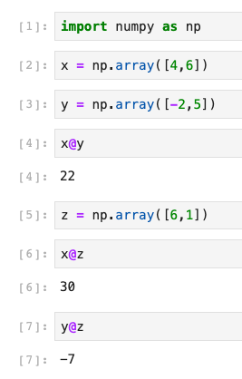
Let’s go back to my simple Perceptron example from a previous blog:

We declared success here when we were able to find a point where the dot product of our weight value (z) and each data point resulted in the proper sign (positive for positive values, negative for negative values.) HOWEVER, we were not using the complete formula for our hyperplane. The full formula is not just z@<data point>, but actually z@<data point> + b. In the example, we simply assumed that our hyperplane crossed through the origin (0,0), and as such, we could just ignore b completely.
In reality, this is not always the case, and not accounting for b when using the Perceptron can result in an algorithm that never solves, even if a hyperplane exists that could separate the data correctly. The question, then, is what is this offset, and how can we account for it?
By trial and error, I figured out that you could test each data point with z@<point> + b (assuming b initially starts at zero), and then for positively labeled values you could add an arbitrary small value to b (I tested values from 0.5 to 2 with success), and for negatively labeled values subtract that same value. If you hit more positive than negative misclassified points, your b would be positive, and if you hit more negative misclassified points, your b would be negative. This made the program work, but it meant keeping track of a b value in a separate thread.
What my wife demonstrated to me this evening was you could simply add your b adjustment value (in the course they used 1 as the example, which makes sense) to each data point as a new dimension, and then instead of keeping b as a separate value, include it as a new dimension in your weight vector. Here’s what that looks like if we adjust the previous example and factor in b to our equation.

Given the random values I chose for my example, this ends up not changing the number of iterations, but in the first example in the class, accounting for the offset **ACTUALLY MAKES YOU GO THROUGH TWO MORE ITERATIONS** compared to what they walk you through in class. (In other words, I believe the in-class example is at best incomplete, and quite possibly incorrect…) In one fell swoop, I now both understood what “absorbing” the b value into the data set meant, how it works when the matrix multiplication is applied, and why they choose 1 as the offset (since it doesn’t appear to matter within a reasonable range, I think it just makes the math easier).
However, this turns out to be an oversimplification. With a little experimentation I figured out that your data values absolutely matter with what “reasonable” for the offset means. For example, you can create conditions for a lot more iterations with an offset too large, and it is also true that “too large” is relative to the values of the data you’re working with in the first place.
Take a look at this example, where I made the data points a little harder to separate and it now takes several steps for my Perceptron to find a hyperplane, using an adjustment value of 1 for b:

Now take a look at what happens when I set my b adjustment to 10 instead of 1:

I believe this Perceptron would eventually reach convergence, but it would take a little while. So for these values, a b value of 1 makes sense. What if, however, our data values were much, much smaller? Does an offset of 1 still make sense?

As you can see, when the values were harder to separate and very very small, a b value of 1 no longer made the same kind of sense. Thus, for optimum effect you would probably need to adjust your b value and scale it to some range that is decently close to the magnitude of the values in your data.
I still have a ways to go, but it was extremely satisfying to go from having figured out how to code but not truly understood something to having a pretty firm grasp on what goes on behind the scenes and why, as well as what situations the in-class instructions apply and which ones they don’t. Hopefully this little walk-through has been helpful for you as well.